Low volatility environments are periods in which price changes remain unusually small relative to an asset’s own history. In technical analysis, the concept is used to interpret market behavior when price variation compresses and trading ranges narrow. Although low volatility often feels calm, it carries its own information about market uncertainty, liquidity, and the balance of buying and selling pressure. Understanding how to identify and contextualize these phases helps analysts read charts more accurately and avoid over-interpreting small price moves.
Defining Low Volatility in Technical Terms
Volatility refers to the magnitude of price variation over time. In practice, technicians frequently operationalize volatility using realized measures derived from historical prices. A low volatility environment is present when those measures fall to the lower end of their recent distribution for a given instrument and timeframe. The definition is inherently relative. A 1 percent daily move may be insignificant for a small-cap biotechnology stock, but large for a short-term government bond ETF.
Several quantitative lenses are commonly used to define “low”:
Rolling standard deviation of returns. Analysts compute the standard deviation of log returns over a rolling window, such as 20 trading days for daily charts. A drop in the rolling standard deviation to a low percentile of its trailing distribution signals a low volatility regime.
Average True Range (ATR). ATR averages the True Range over a set window. True Range captures the maximum of three quantities for each bar: high minus low, absolute value of high minus prior close, and absolute value of low minus prior close. ATR smooths these values to estimate typical range. A sustained decline in ATR, especially when scaled by price level, is a practical indicator of contraction.
Band-based contractions. Indicators that represent dispersion, such as Bollinger Bands or Keltner Channels, visually compress when volatility declines. The width of these bands can be measured explicitly, for example as the ratio of band width to price, and then evaluated against its own history.
Historical volatility (HV). HV annualizes the standard deviation of returns over a window and provides a comparable scale across instruments. Low HV relative to the instrument’s long-run profile flags a quiet regime.
Range-based estimators. Measures that use intraperiod highs and lows, such as Parkinson or Garman–Klass estimators, can diagnose low volatility even when closes appear stable. These measures are helpful if intraday ranges contract.
These tools do not assert direction. They quantify how much price has been moving, not where it will move next.
How Low Volatility Appears on Price Charts
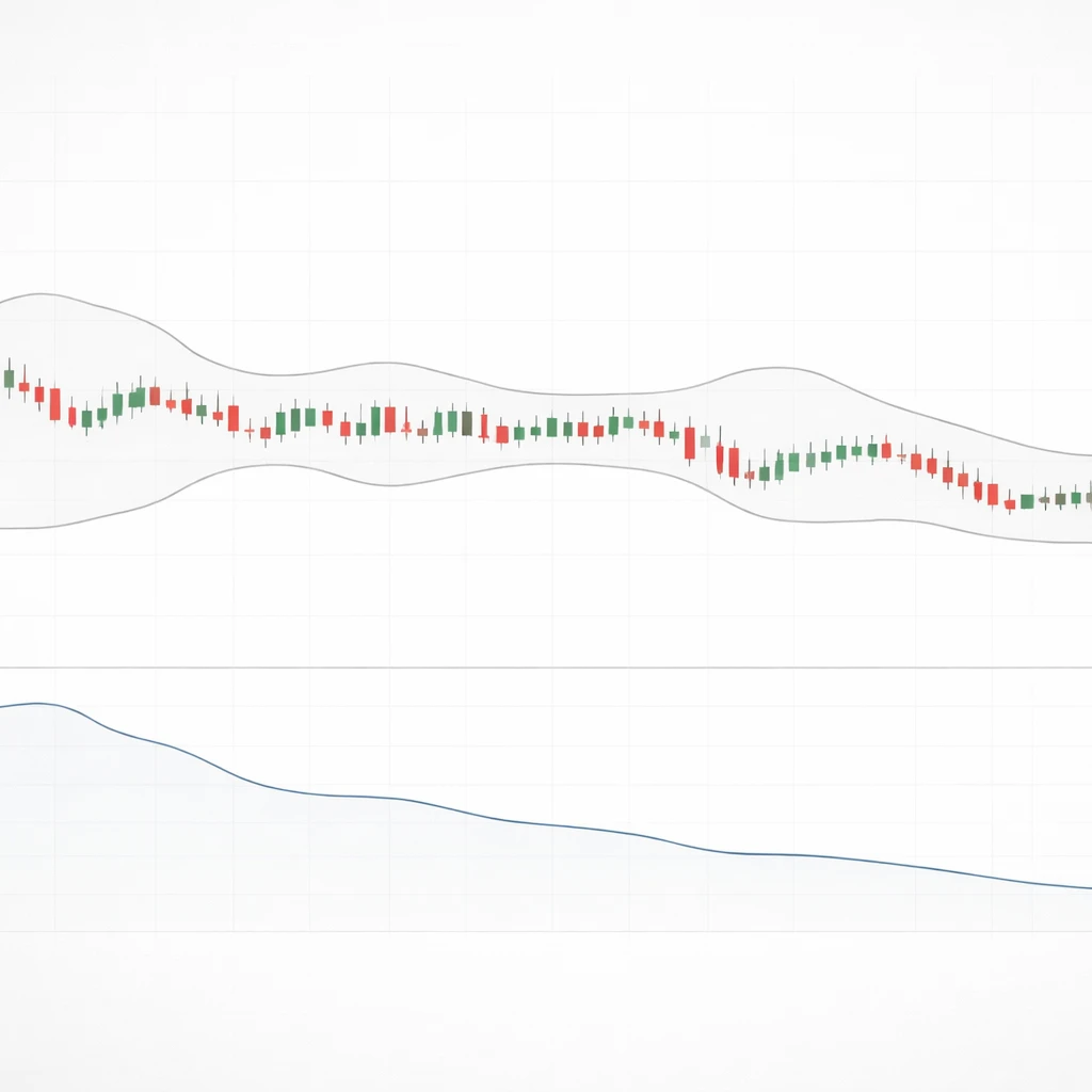
Low volatility often has a distinctive visual signature. The chart appears to “tighten,” with less distance between highs and lows, and frequent overlap from one bar to the next.
Narrow candlesticks and overlapping bars. Consecutive bars with small bodies and relatively short wicks indicate that intraday pushes fail to extend far from the open or prior close. A sequence of such bars aligned near a flat moving average suggests stagnation in the underlying trend’s strength.
Contracted bands and channels. When Bollinger Bands compress around price, the distance between the upper and lower bands shrinks. Keltner Channels may show a similar narrowing. Visual compression is an immediate clue that the standard deviation or range has fallen.
Flattening ATR line. On a sub-chart, the ATR line that once trended higher may roll over and drift lower. The absolute level of ATR matters less than its change relative to recent weeks and its ratio to price.
Sideways consolidation zones. Price can oscillate within a well-defined horizontal box for an extended period. The box’s height, measured in percentage terms, may be smaller than the instrument’s typical short-term range.
Timeframe dependence. A market can be low volatility on the daily chart while intraday action remains active, or quiet intraday while weekly bars are muted. The diagnosis depends on the timeframe the analyst is studying.
Why Traders Pay Attention to Low Volatility
Low volatility environments contain several kinds of informational content that are relevant for interpretation, risk assessment, and context setting in technical work.
Uncertainty can be high even when movement is small. Prices may compress because information is scarce or conflicting, not because risk has vanished. Market participants can be waiting for macroeconomic data, earnings, policy decisions, or seasonal liquidity to return. In such periods, small moves do not necessarily imply confidence or consensus.
Volatility clustering and regime perspective. Volatility tends to cluster. Quiet periods often follow other quiet periods until a shift in conditions occurs. Analysts track low volatility to understand regime duration and the probability that today’s environment will resemble yesterday’s. This is useful for framing expectations about typical range sizes without assuming direction.
Signal reliability and noise. Many technical signals rely on movement of a certain magnitude. When volatility contracts, indicators that were tuned for higher ranges may over-trigger or generate whipsaws. Recognizing a low volatility regime guides the interpretation of indicator behavior.
Liquidity and microstructure. Narrow ranges can coincide with tighter bid-ask spreads and lower depth, or with sufficient depth that price probes fail to travel far. Observing volatility in conjunction with measures of turnover helps distinguish between quiet due to limited participation and quiet due to balanced participation.
Interaction with options markets. If implied volatility diverges from realized volatility, the chart’s quiet appearance gains additional context. A calm price series with elevated implied volatility suggests that option markets expect larger future moves than realized prices currently show. The opposite indicates complacency in expectations or a lack of demand for protection.
Measurement and Interpretation: Practical Tools
Technical analysts typically combine a small set of volatility measures to triangulate a low volatility environment. Each measure carries assumptions and sensitivities.
Average True Range and ATR%. ATR is often scaled by price to form ATR% so that a $2 ATR means different things for a $20 stock compared with a $200 stock. Analysts might examine whether ATR% has fallen below a trailing percentile, such as the 20th or 10th percentile over the past year. The window length matters. Short windows respond quickly but can mislabel temporary dips as regime shifts. Longer windows are steadier but slower to reflect recent changes.
Bollinger Band width and normalized dispersion. Band width is typically a multiple of the standard deviation of recent prices. A straightforward approach is to compute band width divided by the moving average. This normalization enables comparisons across time when price level trends upward or downward. Persistent narrow band width suggests sustained low dispersion in returns.
Historical volatility and rolling windows. HV computed on log returns provides a scale that can be compared across instruments if annualized. The level of HV that qualifies as low depends on the instrument’s long-run profile. A low HV reading for an equity index might still be high for a short-term rate instrument. The window length strongly influences readings; analysts often inspect several windows simultaneously.
Range-based estimators. If a market gaps at the open but trades quietly during the day, close-to-close variance may not fully reflect intraday calm. High-low based measures complement return-based metrics by capturing the intraday spread of prices.
Percentile ranks and z-scores. Because “low” is relative, many practitioners express volatility measures as percentile ranks within a rolling lookback. A reading in the 10th percentile conveys more context than an absolute number. Z-scores serve a similar purpose by showing how many standard deviations a current reading lies below its trailing mean.
Multiple timeframes. Analysts often compute these measures across timeframes. For instance, ATR% may be low on the daily chart while weekly HV remains moderate. The intersection of low and high readings across horizons frames whether the quiet is micro in nature or part of a broader macro lull.
Chart-Based Context: An Illustrative Example
Consider a liquid equity index ETF on a daily chart. Over a six-week span, the daily Average True Range falls from 2.4 percent of price to 1.1 percent. Bollinger Bands set at a 20-day lookback contract until the upper and lower bands are only 2.2 percent apart, compared with a typical 5 to 6 percent range observed earlier in the quarter. Candles overlap for many sessions, with several doji-like bars and few closes near session extremes. A 20-day simple moving average flattens and price oscillates closely around it.
Volume shows a mild decline relative to its 50-day average, though not uniformly. Some sessions print above-average volume without appreciable price progress, indicating rotation among market participants that nets to little directional change. The percentage of days with intraday ranges below 1 percent increases. This combination of compressed price range and mixed volume suggests a market in balance, with sufficient two-sided interest to prevent persistent excursions from the mean.
On a separate intraday perspective, the same instrument during the overnight session exhibits even tighter dispersion. The high-low ranges in the first half of the trading day are modest, followed by slightly wider ranges during the last hour as liquidity thins and closing imbalances develop. The daily context remains low volatility, but intraday nuances reveal when small bursts of activity cluster within the session.
Such descriptive analysis does not prescribe any trading action. It helps an analyst set realistic expectations about typical bar size, the likelihood that small indicator triggers carry weight, and whether price needs a catalyst to expand its range.
Market Microstructure and the Origins of Calm
Low volatility can arise for structural reasons unrelated to conviction about valuation. Several microstructure features are relevant:
Calendar effects. Holidays, end-of-quarter reporting periods, and major data releases can suppress realized volatility as participants delay decisions. The calm may end quickly when scheduled uncertainty resolves.
Order book dynamics. When passive liquidity is abundant at multiple price levels, incremental buying or selling is absorbed without large price impact. The chart registers this as small bars and overlapping sessions. Conversely, fewer firm quotes can still coincide with low volatility if order flow is balanced.
Hedging and cross-asset relationships. If derivatives are actively used to hedge exposures, net directional pressure in the underlying may be muted. At times, cross-asset hedging reduces realized volatility in one market even when related markets move more widely.
Regulatory and index-related events. Rebalances or restrictions can produce predictable supply and demand that offsets during the period, limiting realized moves until the event passes.
Volume Behavior in Low Volatility Environments
Volume often contracts alongside price range, but the relationship is not mechanical. Several volume patterns commonly appear:
Broad decline in turnover. Participation wanes across sessions, especially in the absence of catalysts. The volume moving average drifts lower, and on-balance volume flattens. Price advances or declines during this time tend to lack follow-through.
Rotation without net progress. Volume remains steady, yet price holds within a narrow corridor. This can indicate active sector or participant rotation where buy and sell flows offset. The chart may show alternating small up and down closes, with negligible net movement over several weeks.
Volume spikes that fail to widen ranges. Occasional news items or index-related flows create brief volume surges. If the range remains small despite high turnover, the implication is that liquidity absorbed the shock. The quiet regime persists in realized terms even though participation momentarily increased.
Interpreting volume during quiet regimes helps distinguish between apathy and balance. Neither conclusion dictates direction. Both shape expectations for how easily price might travel if conditions change.
Statistical Properties: Clustering and Persistence
Volatility is well known to exhibit autocorrelation in magnitude. Large absolute returns tend to follow large absolute returns, and small absolute returns tend to follow small ones. This persistence underlies the notion of volatility regimes. In statistical modeling, frameworks such as GARCH or regime-switching models capture this behavior by allowing variance to evolve over time and to depend on its own history.
For the chart reader, the practical implication is that once a low volatility phase is evident, it has a tendency to continue until a new source of information or a shift in participation changes the balance. The duration is highly uncertain, and the end of a quiet regime cannot be timed reliably from volatility measures alone. Nonetheless, the existence of clustering justifies tracking volatility levels as a state variable rather than treating each day’s range as independent from the prior day’s.
Common Pitfalls and Misreadings
Several misconceptions can lead to overconfidence or misinterpretation during low volatility periods.
Equating low volatility with low risk. Small daily moves do not guarantee safety. Price can travel far over time through many small steps. Tail events can also arrive unexpectedly from a calm state.
Assuming imminent expansion. While many market narratives state that quiet leads to storm, there is no fixed cadence. Low volatility can persist for much longer than analysts expect. Forecasting a near-term expansion simply because ranges are small is not reliable.
Overfitting indicator parameters. Retuning indicators to fit a recent quiet patch may produce misleading signals when volatility normalizes. Settings chosen in a low volatility regime may not generalize.
Ignoring the role of price level. If an instrument has trended higher, a fixed-point range measure can understate true contraction or expansion. Scaling volatility measures by price helps maintain comparability.
Neglecting cross-timeframe context. A low volatility day within a high volatility month can be a minor pause, not a regime shift. Conversely, a string of quiet weeks can matter even if a single day shows an outsized move due to idiosyncratic news.
Integrating Low Volatility into Technical Analysis
Analysts can integrate the concept of low volatility into their workflow without venturing into strategy prescriptions.
Expectation setting for range and noise. Recognizing a quiet regime informs expectations about the typical size of intraday or daily moves. This is useful for evaluating whether a small price change carries informational weight or likely falls within noise.
Indicator calibration and interpretation. In low volatility phases, momentum indicators, oscillators, and breakout detectors may trigger frequently with limited significance. An analyst who monitors volatility levels can interpret these triggers with appropriate caution, understanding that smaller swings are typical.
Scenario planning and catalyst mapping. By combining volatility readings with a calendar of potential catalysts, an analyst frames which sessions are more likely to see a change in realized range. This is not a prediction; it is a recognition that scheduled information can alter the balance that sustains quiet conditions.
Backtesting by regime. When evaluating historical behavior of patterns, segmenting the sample by volatility regime often reveals that certain chart behaviors occur with different frequencies in quiet versus active markets. This encourages more nuanced interpretation of signals without implying a course of action.
Transaction cost and slippage assumptions. Quiet markets can exhibit tighter spreads and smaller slippage, though not universally. Risk and cost models that are conditional on volatility regimes better reflect the environment shown on the chart.
Multiple Timeframe Perspective
Volatility is scale dependent. A weekly chart might show a compact series of bars that suggests a broader, low volatility macro environment, while the daily chart still displays intermittent bursts of movement. Conversely, a daily chart can be extremely quiet while an intraday chart appears noisy, because noise at short horizons averages out at daily frequency.
Analysts often cross-check volatility measures across timeframes to avoid mislabeling the environment. A practical approach is to treat low volatility as a nested property: intraday low volatility nested within daily low volatility is stronger evidence of genuine calm than either alone. Disagreement between timeframes, while common, highlights which horizon dominates current market behavior.
Relating Low Volatility to Trend and Structure
Price can be quiet during an uptrend, downtrend, or sideways consolidation. The interaction between trend and volatility informs structural interpretation.
Quiet trending. A steady drift with small bars indicates orderly participation. Moving averages slope gently, and pullbacks are shallow. Despite the calm, such phases can conceal risk if participation is one-sided and susceptible to abrupt rebalancing.
Quiet range-bound behavior. When price oscillates within a narrow horizontal corridor, support and resistance levels appear well defined. The small amplitude encourages frequent tests of boundaries with limited follow-through. The structure reflects equilibrium between buying and selling interest near the mean.
Quiet after a shock. Following a large move, volatility may collapse as the market absorbs new information and reassesses fair value. Price can enter a holding pattern while participants update views. The quiet that follows is not necessarily a reversal or continuation signal; it is a pause in realized dispersion.
Data Quality and Practical Considerations
Accurate assessment of volatility requires attention to data handling.
Corporate actions and roll adjustments. Splits, dividends, and futures contract rolls need to be handled appropriately. Failing to adjust series can distort ATR, band width, and HV calculations, leading to spurious readings of contraction or expansion.
Session definitions. For instruments that trade nearly around the clock, the definition of a trading day matters. Using a continuous session versus a primary exchange session can materially change measured ranges and band compressions.
Outliers and filters. Single-bar anomalies due to bad ticks or one-off prints can skew volatility measures. Applying basic outlier filters or using robust estimators helps prevent misclassification of regimes.
Another Example: Currency Pair on the 4-Hour Chart
A major currency pair on a 4-hour chart trades for two weeks within a 70 pip envelope, whereas prior weeks typically saw 120 to 150 pip ranges over similar spans. The 14-period ATR in pips declines by roughly one third, and band width narrows accordingly. Several bars show wicks in both directions with closes near the midpoint, indicating frequent intrabar reversals without net displacement. Volume proxies, where available, suggest steady but not elevated participation. The pattern aligns with a quiet regime driven by balanced cross-border flows and limited new information.
From an interpretive standpoint, an analyst seeing this compression recognizes that chart signals relying on threshold moves may carry less weight until typical ranges expand. The currency’s sensitivity to scheduled macro releases provides a natural context for when realized volatility might shift, but the timing and direction remain uncertain.
Limitations of Volatility Measures
Volatility indicators summarize complex dynamics into single numbers. They can lag, and in some cases they can obscure microstructure details.
Lag and smoothing. ATR and standard deviation use past bars and often smoothing. By the time they register extreme lows, the compression may already be several weeks old. This is not a flaw so much as a property to be acknowledged.
Sensitivity to lookback. A 10-day window can label a brief quiet stretch as a regime, while a 60-day window may ignore it entirely. Analysts often examine several windows to understand the hierarchy of calm.
Nonlinearity in transitions. The path from quiet to active is not gradual. A single catalyst can overwhelm historical averages in one bar. Measures that assume gradual change may understate the speed of transitions.
Cross-asset comparability. Expressing volatility in percentage terms or annualized units aids comparison, but structural differences remain. Equity index volatility is influenced by earnings and policy cycles. Currency volatility reflects macro data and central bank communication. Commodities often respond to inventory and seasonality. A single definition of “low” cannot fit all.
Using Low Volatility as Context, Not Prediction
Low volatility environments are descriptive states that frame how much price is moving. They are not predictors of direction, and they are not deterministic regarding timing of change. When treated as context, volatility readings improve chart interpretation, help set expectations for typical range sizes, and guide how much weight to place on small price signals. When treated as a forecast in and of themselves, they can invite overconfidence and misallocation of attention.
Key Takeaways
- Low volatility environments are periods when realized price variation falls to the lower end of an instrument’s own historical distribution for a chosen timeframe.
- On charts, they appear as narrow ranges, overlapping bars, compressed bands or channels, and declining ATR relative to price.
- Analysts monitor low volatility to understand regime context, interpret indicator behavior, and set expectations for typical range size without inferring direction.
- Volume can contract or remain steady during low volatility; either way, the interaction between range and turnover refines interpretation of market balance.
- Volatility measures are lagging and sensitive to lookback choices, so they are best used as descriptive context rather than as timing tools.