Technical indicators and oscillators translate raw price or volume data into summarized measures such as trend, momentum, or volatility. Many of these tools move after price has already changed direction. This delay is commonly described as lag. Understanding why indicators lag clarifies what an indicator is measuring, how to interpret it on a chart, and how to set realistic expectations about what an indicator can and cannot convey about current market conditions.
Defining Indicator Lag
Lag is the time delay between a change in price and the response of an indicator that is computed from past prices. When price turns, a moving average typically turns later. When momentum slows, an oscillator such as the Relative Strength Index often shows the loss of momentum only after several bars. This delay is not a flaw in the code. It is a direct consequence of aggregating historical data, smoothing noise, and using definitions that require a window of past observations to be meaningful.
In signal analysis, lag is the shift between an input series and the output of a filter applied to that series. Most technical indicators are filters in this sense. Simple averaging filters reduce noise but introduce a time shift. The more aggressively an indicator suppresses short-term fluctuations, the larger the delay.
Why Indicators Lag at a Mechanical Level
Several design features of indicators produce lag. They often act together, which compounds the delay.
Averaging and Smoothing
Moving averages are the clearest example. A simple moving average uses the arithmetic mean of the last N periods. If price rises steadily for several bars and then falls, the average still contains values from the prior rise, so it turns down only after enough new lower values replace the older higher ones. An exponential moving average reduces the weight on older observations more quickly, but it still blends the past with the present, which cannot be done without some delay.
Oscillators rely on smoothing as well. The RSI computes average gains and average losses over a lookback length, commonly 14 periods. These averages are typically smoothed exponentially. A shift from mostly positive to mostly negative returns takes time to dominate those averages. The effect is a measured response rather than an instantaneous one.
Lookback Windows and Group Delay
Any indicator that uses a window of length N is summarizing the last N observations. In a steady trend, the effective time shift for a simple moving average is roughly half the window length. For example, a 10-period simple moving average often aligns with price action about 5 bars in the past. Exponential averages weight recent data more heavily, which shortens the delay relative to a simple average with the same N, but the lag is still material.
Triangular and double-smoothed averages use multiple passes of smoothing. Each pass adds delay, so the combined filter lags more than a single-pass average. Conversely, shorter windows respond faster because they include less history, but they also admit more noise.
Causality and Close-Based Calculation
Most chart indicators update on the close of each bar. A daily indicator does not know the final value for the day until the session ends. That timing convention adds an additional bar of practical delay in real time. On intraday charts the same logic applies, since the final values only lock at bar close. If the indicator relies on the high or low of the bar, the full range is also known only after the bar completes.
Derived Measures That Layer Lag
Some tools chain smoothing steps, which compounds delay. The Moving Average Convergence Divergence line is the difference between two exponential moving averages. The signal line is another exponential average of that difference. Each stage smooths, and each stage lags. Bollinger Bands use a simple moving average and a standard deviation computed over the same window. Both components depend on the window’s past data, so the bands expand or contract after volatility has already changed.
Noise Reduction Versus Responsiveness
Indicators exist partly to reduce sensitivity to random fluctuations. Reducing sensitivity requires discarding some high-frequency variation. This process cannot separate noise from genuine turning points without delay. There is an inherent trade-off. Less lag means more responsiveness, which admits more false wiggles. More lag means stronger noise suppression, which reduces responsiveness to new information.
How Lag Appears on Charts
Lag is observable once you align price and indicator panels and watch how features in one follow features in the other.
Moving Averages and Trend Lines
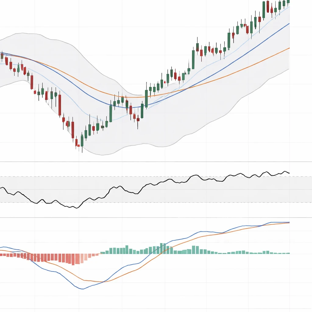
Consider a daily candlestick chart with a 50-period simple moving average. Price forms a V-shaped bottom over five sessions and then rallies. The moving average continues to slope downward for several more days because it still includes the pre-bottom prices. Only after the upward closes dominate the lookback window does the average flatten and then tilt upward. The change in slope is delayed relative to the price trough.
On crossovers the effect is similar. A 50-period average crossing a 200-period average confirms that the shorter window has moved sufficiently above the longer one. That state emerges after a prolonged relative shift. Crossover points typically appear well after the initial price move that set them in motion.
Oscillators and Momentum Panels
Oscillators aim to quantify the rate and persistence of price changes. Their turning points lag for the same reason.
With RSI, a sharp rally from an oversold condition may lift the oscillator out of the lower zone only after several strong closes. Momentum has already improved by the time the oscillator prints a clear change. On the MACD histogram, bars may continue shrinking toward zero even after price has already paused, reflecting the fact that the difference between the fast and slow averages is narrowing but has not yet flipped.
Stochastic oscillators compare the current close to the recent high-low range. If range expands because of a large bar, the oscillator may remain pinned near extremes while price consolidates. The indicator relaxes only as new bars alter the composition of the window.
Volatility and Range Measures
Indicators that measure volatility also lag. Average True Range is a moving average of true ranges, so a large gap day boosts the average for many bars afterward. Bollinger Bands widen after volatility expands, and they remain wide until quiet bars replace the earlier active ones in the calculation window. When observing a squeeze, the contraction reflects a sustained period of low variability that has already occurred.
Volume-Related Indicators
On Balance Volume and moving averages of volume aggregate past flows. A surge in volume shifts these lines, but the smoothing steps afterward keep the indicator elevated or depressed for a while. Subsequent moderate sessions are required before the indicator reverts toward prior levels.
Mathematical Intuition for Delay
The lag of a filter can be described without heavy mathematics. A simple moving average of length N can be viewed as a uniform filter that averages N adjacent samples. In a steadily increasing series, the center of mass of that window sits around the midpoint of the window. That midpoint is about (N minus 1) divided by 2 periods behind the last observation. This is why a 20-period simple average tends to reflect price conditions roughly 10 bars in the past.
An exponential moving average uses a weighting factor often denoted alpha. A common convention sets alpha equal to 2 divided by N plus 1. With that mapping, the effective delay of the exponential average is approximately (N minus 1) divided by 2, slightly less in practice because the weighting never fully discards older data. This is one reason chart users sometimes select an exponential average for faster adaptation. The core trade-off remains. Any smoothing that cuts noise will shift the signal in time.
Oscillators simply extend these ideas. RSI calculates average gains and losses using exponential smoothing. A length of 14 implies that several bars of new information are needed before the average changes meaningfully. MACD uses two exponential averages with different lengths, then applies a third exponential average to the resulting difference. Each layer produces a bounded but real delay.
Standard deviation is also computed over a window. Even if price variability drops abruptly, the standard deviation over the last N bars will decrease only as the older high-variance bars fall out of the window. That is why volatility bands and range averages tend to look slow relative to current candles.
Why Traders Pay Attention to Lag
Lag is often discussed in a negative light, but the delay serves a purpose. Many traders and analysts value lagging indicators because they describe persistent conditions rather than reacting to every fluctuation. The interpretive benefits include the following.
- Context. Smoothed lines and oscillators summarize the recent environment, which helps separate a structural change from a single bar anomaly.
- Comparability. Using fixed lookback windows creates consistent measurements over time and across assets. A 20-period average on one chart is comparable to a 20-period average on another, within each timeframe.
- Confirmation. Delayed responses can corroborate that a change in character has continued long enough to be measurable, which is different from trying to pinpoint the first moment of a turn.
- Communication. Lagging measures provide common reference points such as slopes, crossovers, and band widths that are easy to compare across charts and timeframes.
- Smoothing for analysis. By reducing high-frequency variation, lagging indicators make it easier to examine multi-week or multi-month tendencies without being distracted by intraday or single-session noise.
Understanding that lag is built in helps prevent misinterpretation. If a moving average flattens, it may be reflecting weakness that has already unfolded. If an oscillator leaves an extreme, it may be describing stabilization rather than predicting continuation. Recognizing the descriptive nature of these tools is central to using them appropriately.
Practical, Chart-Based Context
Several concrete scenarios illustrate how lag shows up in daily analysis.
Example 1. Moving Average Response After a Sharp Reversal
Imagine a stock that falls for six sessions and then posts three strong bullish days. A 20-period simple moving average continues downward during the first two up days because 18 of the 20 values in the window are still from the decline. On the third up day the average may flatten, and only after a few more positive closes does it tilt upward. When viewed on a chart, the moving average appears to ignore the reversal at first. In reality it is integrating the recent past into a single line that cannot pivot until the window’s composition changes enough.
Example 2. RSI Emerging From Oversold Conditions
Consider a 14-period RSI on a currency pair. Price registers a sequence of small advances following a selloff. The oscillator may remain below the midpoint for a while, even as price trends upward. The reason is arithmetic. Average losses from the selloff are still part of the denominator, and the new gains need several bars before they outweigh the earlier negatives. When RSI eventually moves above the midpoint, the price advance has already been underway for some time.
Example 3. MACD Histogram and Momentum Slowdown
On an index future, suppose the fast and slow exponential averages have diverged for weeks. Price then pauses and begins to drift sideways. The MACD line starts to approach the signal line as the rate of change slows. The histogram bars shrink, but they may remain above zero for many sessions. Price hesitated first. The indicator confirmed that the difference between the averages was compressing only after enough sideways action accumulated.
Example 4. Volatility Bands After a Breakout
On a daily chart with Bollinger Bands using a 20-period simple moving average and two standard deviations, a breakout day produces a wide candle. The upper band expands within a few bars, and the lower band drops as the standard deviation increases. Even if price calms, the bands stay wide for several sessions because the large breakout candle remains inside the lookback window. Only when that bar ages out do the bands contract noticeably. The band shape lags the volatility event.
Example 5. ATR After a Gap
Suppose a stock gaps down by 4 percent on earnings, creating a large true range. The Average True Range rises immediately and then declines slowly, often over a couple of weeks, as the exceptional bar continues to influence the 14-period average. On the chart the ATR line looks sluggish compared with the daily ranges that follow, which is characteristic of a smoothed volatility measure.
Distinguishing Lag From Repainting
Lagginess should be separated from the concept of repainting. A lagging indicator updates based on available data and does not change its historical values once a bar closes. A repainting indicator revises previously plotted values when future data arrive. Many classical tools such as moving averages, RSI, MACD, and ATR do not repaint. They may be delayed, but once a bar is final the indicator value at that bar is fixed. Some centered filters, such as a centered moving average that uses future bars to position the line exactly under the window’s midpoint, can look very fast in hindsight because they place smoothed values in the center of the window. Those methods are non-causal in real time and are not directly comparable to the standard lagging tools used during live analysis.
Timeframe Effects
The same indicator will exhibit different practical lag depending on timeframe. On a one-minute chart, a 20-period average captures 20 minutes of data and may respond within a short intraday interval. On a weekly chart, a 20-period average summarizes roughly five months, so the delay relative to a new weekly move is substantial. The perception of lag increases with timeframe because each bar itself aggregates more information. This is also why multi-timeframe comparisons require care. A daily moving average of 20 periods and a weekly moving average of 20 periods represent very different horizons.
Parameter Choices and the Lag-Noise Trade-off
Indicator parameters define the balance between stability and responsiveness.
- Longer lookbacks increase lag and usually produce smoother lines.
- Shorter lookbacks reduce lag and increase sensitivity to noise and whipsaws.
- Exponential weighting shortens lag relative to simple averaging at the same nominal length but still lags materially.
- Double smoothing and signal lines add clarity but stack delays.
- Price basis matters. Using the typical price, defined as the average of high, low, and close, often produces smoother results than using close alone, which subtly increases lag.
There is no setting that eliminates lag without consequences. Zero-lag variants exist that attempt to compensate for delay by combining shorter and longer averages. These methods often increase overshoot or sensitivity to abrupt fluctuations. The constraint is fundamental. Any process that filters noise inevitably sacrifices timeliness.
Reading Indicators With Lag in Mind
Recognizing that an indicator describes recent history rather than predicting the next bar helps anchor interpretation.
When a moving average flattens, it means the recent data in the window have balanced out the earlier trend. When an oscillator leaves an extreme, it means the balance of gains and losses has shifted for long enough to change the average. When volatility bands expand, it reflects range dispersion that has already worked through multiple bars. Treating these changes as descriptive prevents overconfidence in a single moment on the chart.
Intrabar behavior is another timing consideration. An indicator that updates on close will not reflect an intraday reversal until the bar completes. A trader viewing the chart mid-bar may see price surging while the indicator remains unchanged. The gap closes at bar close when the final price is incorporated.
Common Misconceptions About Lag
Several misunderstandings recur in discussions of indicator delay.
- Lag is not a programming error. It is a property of smoothing and windowing.
- Lack of lag does not guarantee usefulness. An unsmoothed measure can be timely but dominated by noise.
- Lagging does not imply backward-looking irrelevance. A measured description of recent conditions is often the point of the tool.
- Lag differs from repainting. Most standard indicators are causal and do not retroactively change past values.
- Parameter changes do not create predictive power. They shift the balance between noise suppression and delay.
How Understanding Lag Helps Interpretation
Knowledge of lag supports disciplined reading of chart evidence.
- It clarifies why a confirmation often arrives after a price move. The indicator must accumulate enough new data to outweigh the past.
- It sets expectations for how quickly a line or oscillator will respond after a turning point. A 50-period average will not pivot within a few bars of a sharp reversal.
- It helps diagnose apparent contradictions between price and indicator. Price may surge while a slow indicator barely moves because the window is dominated by earlier data.
- It informs comparisons across instruments and timeframes. The same parameter means different practical delays depending on bar duration and volatility.
- It encourages disciplined interpretation of divergences, crossovers, and band behavior as descriptive context rather than as precise timing cues.
Illustrative Walk-Through: From Price Shock to Indicator Response
To see the sequence in action, imagine a market with these stages.
Stage 1. A two-week decline sets a persistent negative drift. Short-term candles are mostly red. The 20-period simple moving average slopes downward, RSI sits below the midpoint, and ATR gradually rises as ranges widen during the selloff.
Stage 2. A strong reversal day appears, followed by two steady advances. Price has pivoted. The moving average remains downward-sloping because the window is still dominated by the two-week decline. RSI lifts, but remains below its midpoint because recent losses continue to weigh on the smoothed averages. ATR stays elevated, reflecting the cumulative wide ranges.
Stage 3. Several more sessions of stabilization follow. The moving average begins to flatten as new bars replace earlier declines in the window. RSI crosses its midpoint as the balance of gains and losses shifts. ATR edges lower as the largest ranges roll out of the calculation.
Stage 4. Weeks later, the moving average trends upward, RSI spends more time above its midpoint, and ATR has normalized. Every indicator’s state is consistent with a change that started many bars earlier. On the chart the delayed responses are clear. Price turned first, then momentum measures adjusted, and finally longer averages and volatility metrics aligned with the new environment.
Limits of Compensation Techniques
Analysts sometimes seek to counteract lag by differencing indicators or using higher derivatives such as rate of change of an average. These approaches can be useful for sensitivity analysis, yet they replace time delay with increased volatility in the derived line. The histogram of MACD is a familiar example. It responds earlier than a signal-line crossover, but it also oscillates more quickly and can swing through zero multiple times during consolidation. The underlying principle remains intact. Faster response comes with greater variability and a higher likelihood of reacting to transitory noise.
Putting Lag in Perspective
Indicators and oscillators compress information. Lag is the cost of compression that favors stability. On a chart this cost appears as late turns, late confirmations, and measures that change only after the market has moved. Recognizing that pattern aligns expectations with the tool’s design. Indicators do not foretell the next bar. They quantify what has just happened in a way that attempts to filter out randomness and express structure.
Key Takeaways
- Lag arises from smoothing, windowing, and close-based timing that make indicators descriptive rather than instantaneous.
- On charts, lag appears as moving averages turning after price pivots, oscillators confirming momentum changes late, and volatility measures adjusting slowly.
- The lag-noise trade-off is fundamental. Less delay means more sensitivity to noise, while more smoothing increases delay.
- Understanding lag improves interpretation by setting realistic expectations about timing and by clarifying the role of indicators as summaries of recent conditions.
- Most standard indicators lag without repainting. Their historical values are fixed once a bar closes, even though their responses are delayed.