Risk management begins with the recognition that survival is not automatic. In markets, the combination of uncertainty, variance, and finite capital creates the possibility that losses accumulate to a level where activity must stop. The term risk of ruin formalizes that possibility. It is a probabilistic assessment that an account will hit a level of capital from which continuation is not feasible. Understanding risk of ruin reframes decisions about position sizing, leverage, and time horizon around a single idea: capital preservation is a precondition for any long-term process of compounding.
What Risk of Ruin Means
Risk of ruin is the probability that capital falls to a predefined lower boundary. That boundary can be different across contexts:
- Absolute ruin: equity reaches zero. This is a theoretical limit that can occur in highly leveraged or unhedged positions.
- Operational ruin: equity falls to a level that triggers margin calls, exchange liquidation, or broker-imposed restrictions.
- Economic ruin: equity drops below the capital level required to implement a process in a meaningful way, such as the minimum lot size or the reserve capital a risk policy demands.
- Psychological ruin: a drawdown that leads the trader to stop, even if continuation is financially possible.
These boundaries are different expressions of the same structure. A stochastic process evolves over time. It has an absorbing barrier at or above zero. The risk of ruin is the probability that the process will eventually touch that barrier.
Why Risk of Ruin Is Central to Capital Preservation
Return statistics do not guarantee survival. A process can have positive expected return and still have a high probability of hitting a ruin threshold if variability is large relative to capital and position sizes. The arithmetic of compounding amplifies this point. Losses reduce the base from which future gains are measured. A 50 percent loss requires a subsequent 100 percent gain to get back to even. If ruin occurs first, there is no opportunity to compound at all.
Thinking in terms of ruin shifts focus from average outcomes to path dependence. Two strategies with identical long-run average returns can have very different survival profiles if one has fatter tails, more serial correlation in losses, or more leverage. Capital preservation is not achieved by aiming for high average returns. It is achieved by controlling the probability of adverse paths that intersect a capital boundary.
Drawdowns, Volatility, and Path Dependence
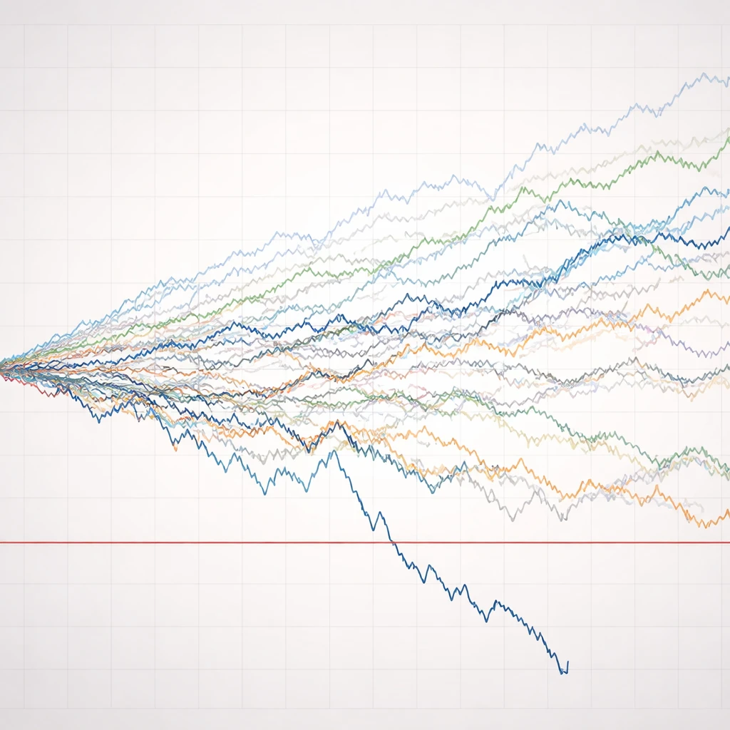
Drawdown is the peak-to-trough decline experienced by an equity curve. Drawdowns describe realized paths. Risk of ruin concerns potential paths that could intersect a boundary. The two are connected but not identical. A strategy that frequently experiences modest drawdowns might have a low risk of ruin if position sizes are small and the distribution lacks heavy tails. Another strategy might show long periods of small, steady gains followed by rare, severe losses that overwhelm capital. The latter can display gentle drawdowns until the day it does not. Its risk of ruin can be materially higher despite a benign history.
Path dependence is the reason. Compounding multiplies returns through time in the order they occur. Sequences with clusters of losses, even if the average is acceptable, can push equity below a boundary before any eventual rebound. Human and institutional constraints add further path dependence. Margin requirements, stop-loss rules, and mandate limits can convert a temporary drawdown into operational ruin.
A Simple Probabilistic Lens
To build intuition, start with a stylized model. Suppose outcomes arrive as independent trials. Each trial is a win with probability p and a loss with probability q = 1 − p. Profit on a win is R units for every unit risked, and the loss is one unit when a loss occurs. This captures the pair of inputs that most trading processes eventually reduce to: win probability and payoff ratio.
There are two common sizing rules in this context.
- Fixed unit sizing: each trial risks one unit of capital. The account moves up or down by one unit at each step. This resembles the classical gambler’s ruin setting.
- Fixed fractional sizing: each trial risks a fixed fraction f of current equity. Gain on a win is f × R of equity, and loss on a loss is f of equity. The account compounds multiplicatively.
Both models are idealizations. Markets exhibit dependence, changing distributions, and variable payoffs. Still, they provide clear insight into how edge and sizing interact to produce or avoid ruin.
Gambler’s Ruin Intuition
Under fixed unit sizing with a favorable edge, the classical result states that the probability of eventually going broke declines exponentially with the number of units of starting capital. If the win probability p exceeds q, and you start with i units while the market or counterparty has effectively infinite capital, then the probability of eventual ruin is approximately (q ÷ p) to the power i. If p is less than or equal to q, the probability of ruin is 1 in the long run.
This result is instructive for two reasons. First, the difference between p and q matters a great deal. A small edge requires many units of capital to make ruin unlikely. Second, capital measured in units of loss is the relevant quantity. Starting with more units or risking smaller units each time is mathematically equivalent in this simple model.
Consider two numerical illustrations, using i to denote starting units:
- If p = 0.55 and q = 0.45 with i = 10, the ruin probability is approximately (0.45 ÷ 0.55) raised to the 10th power, close to 0.134. Ten units at a 55 percent hit rate still leave a measurable chance of going broke in an open-ended sequence.
- If p = 0.52 and q = 0.48 with i = 10, the ruin probability is roughly (0.48 ÷ 0.52) to the 10th power, about 0.45. A small change in edge doubles or triples the chance of ruin if capital is not scaled accordingly.
Trading does not usually operate in unit steps, but the lesson carries over. Edge, measured as the relationship between win probability and payoff ratio, and the amount of capital at risk per trial, jointly determine the chance of hitting a boundary.
Fractional Sizing and Streaks
With fixed fractional sizing, equity evolves multiplicatively. After one loss, equity is multiplied by (1 − f). After k consecutive losses it is multiplied by (1 − f) to the power k. Suppose the ruin boundary is defined as a fraction L of the starting equity. To reach that boundary exclusively through consecutive losses requires at least k losses, where k is the smallest integer satisfying (1 − f) to the power k ≤ L.
This provides a concrete way to relate position size to streak risk. For example, if f = 0.02 and the boundary L is 0.50 of starting capital, then k must be at least ln(0.50) ÷ ln(0.98), which is about 34.3. That means 35 consecutive losses would halve the account. If the probability of a loss on any given trial is q, the probability of 35 losses in a row is q raised to the 35th power. For moderate q, that event is extremely unlikely. If f = 0.10 with the same L, then k is ln(0.50) ÷ ln(0.90), roughly 6.6. Seven losses in a row would cut the account in half. If q is 0.60, the probability of seven losses in a row is 0.6 raised to the 7th power, about 0.028. Consecutive-loss paths become much more plausible at larger f.
Consecutive losses are a simplified lens. In practice, drawdowns arise from clusters of losses and small gains that fail to offset them. Over many trials, the probability of encountering at least one long streak is higher than the probability computed for any single block. The longer the horizon, the more likely it is that an adverse run occurs at some point. Fixed fractional sizing is valuable because it scales risk with equity, but it does not eliminate the possibility of touching a boundary if f is large relative to the process variance.
How Risk of Ruin Appears in Real Trading
Market structure, instruments, and constraints shape where the ruin boundary sits and how quickly a path can hit it. The mechanisms differ across contexts, but the underlying drivers are consistent: leverage, variance, and the correlation of adverse outcomes.
Leverage, Margin, and Forced Exits
Leverage alters the mapping between price moves and equity moves. A highly leveraged position can turn a routine price fluctuation into a large percentage change in account equity. Margin rules add an operational boundary that may be reached well before equity would mathematically trend toward zero. For example, an account that uses futures or CFDs can be liquidated by the broker if equity falls below maintenance margin, even if the underlying position might have recovered. In this setting, the ruin boundary is the maintenance threshold. Risk of ruin becomes the probability that the equity path hits that level during the life of the position or across a sequence of positions.
Concentration and Correlated Losses
Adding positions does not automatically reduce risk of ruin. If positions are highly correlated or tied to the same risk factor, losses tend to cluster. A portfolio of similar trades can experience a joint drawdown that looks like a single large position. Measured independence matters. The benefit of diversification in lowering ruin comes from holding risks whose adverse outcomes are less likely to occur at the same time.
Liquidity, Slippage, and Gap Risk
Estimates of ruin that ignore market frictions tend to be optimistic. Stop orders can execute at worse prices in fast markets. Overnight gaps and event risks create discontinuous moves. Option sellers can experience large losses from rare events that do not resemble the average day. In these environments, the payoff distribution is skewed, and the tail may be fatter than a Gaussian model implies. The chance of a single step that jumps directly to or through the boundary is not captured by models with small, frequent steps.
Estimating Risk of Ruin
Estimation involves specifying a return process, a position sizing rule, and a boundary. Different approaches are available, each with its own assumptions and limitations.
Analytical Approximations
Closed-form results exist only for simple processes. The classical gambler’s ruin formula applies to unit-step processes with constant win probability and loss probability. For fractional sizing and variable payoffs, log-utility and growth-optimal frameworks study conditions for positive long-run growth. A common criterion is that the expected value of the log of the growth factor is positive. Formally, one asks whether p × log(1 + fR) + q × log(1 − f) is greater than zero for a given f. When this expression is negative, the process drifts toward ruin in a multiplicative sense. When it is positive, the process grows on average, but the chance of hitting a boundary before growth is nonzero if f is large or tails are heavy.
Analytical formulas teach directionality. Risk of ruin typically decreases when the edge improves, when position sizes shrink, when volatility declines, and when outcomes are less correlated. They also show that small changes near breakeven can have large effects. Moving from p = 0.50 to p = 0.52 with symmetric payoffs changes the long-run character of the process. Whether that change translates into a low probability of hitting a finite boundary depends on capital and sizing.
Monte Carlo Simulation
When distributions are complex, simulation is a practical tool. A representation of returns is sampled repeatedly to produce many equity paths under a chosen sizing rule. The fraction of paths that cross the boundary within a specified horizon provides an empirical estimate of risk of ruin over that horizon. Simulation is flexible. It can incorporate fat tails, serial correlation, time-varying volatility, and liquidity-induced jumps. It can also reflect operational constraints such as margin calls. The validity of the estimate depends on how well the simulated process matches the actual one. Model error and regime changes remain important caveats.
Scenario analysis is a related technique in which rare but plausible shocks are injected into simulated paths. This highlights sensitivity to tail events that are underrepresented in short samples. For example, adding periodic large gaps consistent with historical crisis periods can change the estimated probability of touching the boundary even if day-to-day volatility is unchanged.
Choosing and Interpreting Boundaries
Ruin is not always absolute. Practical risk management often defines a stop level for a strategy, a drawdown budget for a fund, or a regulatory limit that functions as an absorbing barrier. The chosen boundary expresses risk tolerance and operational reality. A 20 percent boundary will by construction produce higher estimated risk of ruin than a 50 percent boundary, all else equal. The appropriate boundary depends on instrument liquidity, leverage, mandate requirements, and the capacity to continue after losses. Interpreting estimated ruin probabilities requires clarity about which boundary is being referenced and over what horizon.
Common Misconceptions and Pitfalls
Several errors recur when practitioners think about ruin.
- Confusing average return with survivability. A positive average does not prevent a low but nonzero chance of an adverse path that crosses the boundary. Survivability depends on variability and sizing.
- Ignoring heavy tails and jumps. Gaussian approximations understate the chance of large, discrete moves. Instruments exposed to gap risk or event risk are particularly vulnerable.
- Assuming independence. Losses can cluster due to common risk factors, crowded positioning, or volatility regimes. Independence assumptions inflate diversification benefits and understate ruin probabilities.
- Overfitting edge estimates. Estimating p and R from short samples and then plugging them into formulas can create misplaced confidence. Sampling error and regime shifts can reduce or eliminate the perceived edge.
- Neglecting operational thresholds. Margin rules, minimum trade sizes, or investor drawdown limits can force exits before mathematical ruin. A realistic model must include those thresholds.
Risk of Ruin, Drawdowns, and Recovery
Drawdowns shape both the probability of ruin and the time to recover. The relationship between drawdown and recovery is asymmetric. After a 10 percent drawdown, the required gain to recover is approximately 11.1 percent. After a 50 percent drawdown, the required gain is 100 percent. As drawdowns deepen, the recovery requirement accelerates. This is a core reason capital preservation dominates: avoiding deep drawdowns reduces the horizon required for recovery, even if the average return is unchanged.
In this light, risk of ruin is best viewed as a probability that depends on three levers: the distribution of outcomes, the fraction of capital risked, and the placement of the boundary. Changing any one of them changes the distribution of drawdowns and the likelihood of reaching an absorbing threshold.
Applications Across Trading Styles
Different trading styles face distinct versions of ruin risk.
- Short-horizon leveraged trading. High turnover and leverage can put the ruin boundary near the current equity level because maintenance margin is an operational floor. Even small adverse runs can trigger forced exits if position size is large relative to capital.
- Directional option selling. Many small gains offset by rare large losses produce distributions with high skewness. The win rate can be high while the risk of a catastrophic gap that reaches the boundary in a single move remains material.
- Multi-asset portfolios. Apparent diversification can vanish in crises if correlations spike. Estimating ruin requires modeling correlation dynamics, not just average correlations.
- Unlevered long-only investing. Even without leverage, economic or psychological boundaries exist. For example, a mandate may stipulate that a strategy stops at a 25 percent drawdown. Risk of ruin then means the chance of violating that limit over a given horizon.
Practical Interpretation Without Recommendations
The concept of risk of ruin is descriptive, not prescriptive. It quantifies how likely it is that a specific configuration of edge, volatility, and size will intersect a boundary within a defined horizon. Its primary value is diagnostic. It highlights whether a process is fragile to adverse sequences and whether the tolerance for drawdown aligns with the behavior of the underlying distribution. That diagnostic perspective supports disciplined capital preservation by making the trade-off between growth and survival explicit.
Two further points help with interpretation. First, risk of ruin is horizon dependent. Over a longer horizon, there are more opportunities for adverse sequences to occur, so the probability of touching the boundary typically increases. Second, risk of ruin is sensitive to model choice. Estimates that exclude jumps, regime shifts, or correlation changes are often lower than what real-world conditions produce. Stress testing across a range of assumptions provides a more informative picture than a single point estimate.
Worked Example: From Inputs to Ruin Probability
To connect the pieces, consider a simplified worked example with a fractional sizing rule. Suppose a process has p = 0.45, q = 0.55, and R = 2.0. The expected gain per trial is positive in a loose sense because wins are larger than losses. However, the distribution is volatile. Let the sizing fraction be f = 0.04. Define the boundary L as 0.50 of starting equity. The minimum number of consecutive losses needed to hit the boundary is k = ln(0.50) ÷ ln(0.96), approximately 17.7, so 18 consecutive losses would halve the account. The probability of 18 losses in a row is 0.55 raised to the 18th power, around 0.0008.
This seems small, but the horizon matters. Over 5,000 trials, the probability of encountering at least one 18-loss streak is not simply 0.0008. The chance of at least one occurrence grows with the number of overlapping blocks where such a streak could begin. In addition, real drawdowns rarely occur as clean streaks. Clusters and partial recoveries can still push the path below the boundary with similar or higher probability. If f increases to 0.08, k becomes ln(0.50) ÷ ln(0.92), close to 8.3, so 9 consecutive losses are sufficient. The probability of at least one 9-loss run over a long horizon is materially larger.
Now change the boundary to represent margin-induced operational ruin. Imagine maintenance margin implies that a 30 percent drawdown leads to liquidation. With f = 0.08, the minimum consecutive losses to hit 0.70 is k = ln(0.70) ÷ ln(0.92), near 3.9. Four consecutive losses would be enough. In a process with q = 0.55, the probability of four losses in a row is 0.55 raised to the 4th power, approximately 0.0915. Over many sequences, the chance of at least one such cluster becomes significant. This shows how raising f or lowering the boundary can transform a process from resilient to fragile even without changing p or R.
What Low Risk of Ruin Implies
When a configuration of edge, variance, and size yields a low ruin probability for a given boundary and horizon, it implies that the equity path has a high likelihood of staying within a tolerable drawdown range. It does not imply that returns will be high, that drawdowns will be comfortable, or that tail events are impossible. It means only that crossing the specified boundary is unlikely under the modeled distribution. That distinction matters whenever results are evaluated. Survival is necessary for compounding, but it is not sufficient for attractive performance.
Limitations and Sensitivities
Every estimate of risk of ruin inherits assumptions. Stationarity is the most important. If p and R are estimated from past data but the process changes, the estimate can be misleading. Serial correlation and volatility clustering can raise ruin probabilities relative to independent-trial models. Liquidity effects, slippage, and fees reduce effective edge and can turn a borderline process into one with meaningful ruin risk. The placement of the boundary is also a judgment call. Setting it too high may overstate ruin in contexts where temporary drawdowns are tolerable. Setting it too low may understate operational risk in leveraged settings.
Final Perspective
Risk of ruin is not an abstract curiosity. It is the mathematical articulation of a simple constraint: capital must remain intact enough to continue. An account that repeatedly avoids large drawdowns gains time for edges to express themselves. An account that occasionally crosses a boundary may never realize any long-run average because activity stops. Recognizing this shifts attention from maximizing average returns to understanding how size, variance, and tail risk interact with the capital base. That understanding is the foundation of prudent capital preservation.
Key Takeaways
- Risk of ruin quantifies the probability that an equity path hits a capital boundary where continuation is not feasible, whether absolute, operational, economic, or psychological.
- Survivability depends on variance, tail risk, and position size relative to capital, not on average returns alone.
- Simple models show ruin probability falling with stronger edge and smaller units of risk, but real markets add jumps, correlation, and regime shifts that raise practical ruin risk.
- Fractional sizing scales risk with equity, yet large fractions can still lead to boundary crossings through plausible clusters of losses.
- Estimates are model dependent and horizon dependent; stress across assumptions and boundaries provides a more informative view than any single point estimate.